
How to Categorize Transactions Automatically
Add a Rules tab that maps a keyword to a category, then use one lookup formula in your Transactions tab that scans each bank description for the first matching keyword. Drag it down once and every transaction categorises itself — including the ones you paste in next month.
This is the single biggest time saving available in a budget spreadsheet. Logging an expense stops being "type the amount, then pick the category" and becomes "paste the bank export". The categories fill themselves in.
Step 1: The Rules tab
Add a third tab called Rules. Two columns: a keyword that appears in your bank's description text, and the category it should map to.
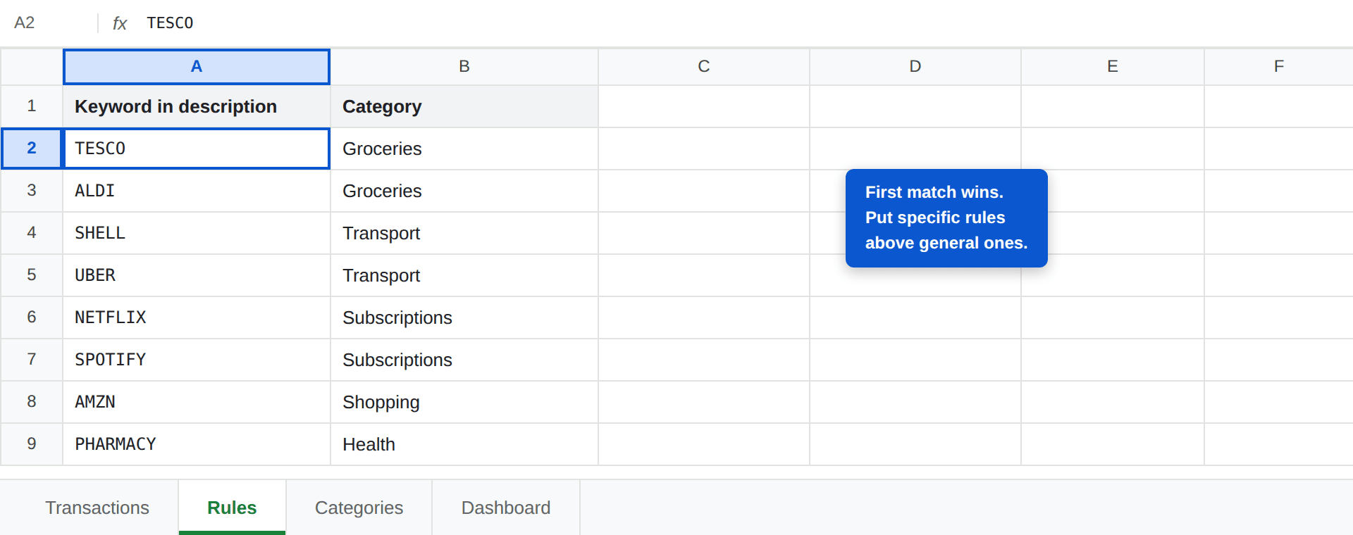
Keywords come from the descriptions your bank actually writes, not from what you'd call the shop. Open a recent export and copy the distinctive fragment: TESCO STORES 3421 becomes a rule of TESCO; UBER TRIP HELP.UBER becomes UBER. Short and distinctive beats long and exact, because the trailing reference numbers change every time.
Ten to fifteen rules will usually cover 80% of a normal month. You are not trying to be exhaustive on day one.
Step 2: The formula
In the Transactions tab, put this in the Category column — assuming descriptions are in column D:
=IFERROR(INDEX(Rules!$B:$B, MATCH(1, ARRAYFORMULA(ISNUMBER(SEARCH(Rules!$A:$A,$D2))*(Rules!$A:$A<>"")), 0)), "Uncategorised")
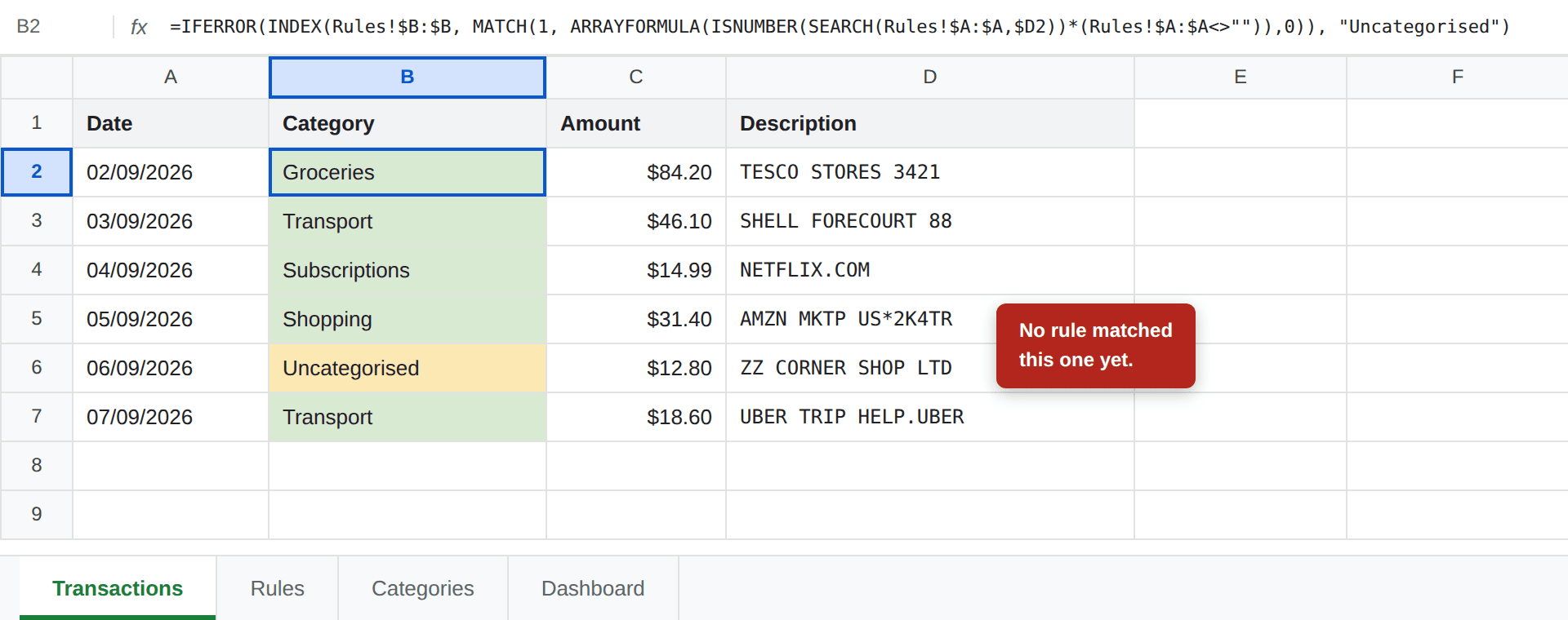
Reading it from the inside out:
SEARCH(Rules!$A:$A, $D2)looks for every keyword inside this row's description, returning a position or an error for each.ISNUMBER(...)turns that into TRUE/FALSE — found or not found.MATCH(1, ..., 0)finds the first match in the list.INDEX(Rules!$B:$B, ...)returns that rule's category.IFERROR(..., "Uncategorised")catches the case where nothing matched.
ARRAYFORMULA is what makes Sheets evaluate the whole rules column at once instead of just the first cell. Leave it out and the formula silently only ever tests your first rule.
The blank-row bug
Most versions of this formula you'll find online look like this, without the extra multiplication:
=IFERROR(INDEX(Rules!$B:$B, MATCH(1, ARRAYFORMULA(ISNUMBER(SEARCH(Rules!$A:$A,$D2))), 0)), "Uncategorised")
It works right up until it doesn't. SEARCH("", anything) returns 1 — an empty keyword matches every description at position 1. Because you referenced the whole column, the first blank row under your last rule matches everything.
The symptom is subtle and that's what makes it nasty: transactions that should say Uncategorised come back blank instead, because they matched a blank rule and returned its blank category. Nothing errors. Your dashboard just quietly loses those rows, and if you've read why SUMIFS stops adding up, you'll recognise the shape of the problem.
The fix is the *(Rules!$A:$A<>"") in the working version above. Multiplying TRUE/FALSE by TRUE/FALSE gives 1 only where the keyword both matched and isn't blank — which is why that version uses MATCH(1, ...) rather than MATCH(TRUE, ...).
Run your numbers
Budget template
Three tabs with live formulas — add a Rules tab and this drops straight in.
Make a copy →Budget Calculator
Set the category budgets your dashboard will measure against.
Open calculator →Ordering: first match wins
MATCH stops at the first hit, so the order of your rules is the logic. Specific rules go above general ones:
AMZN MKTP→ Shopping (row 2)AMZN→ Subscriptions (row 8)
Marketplace purchases hit the first rule; Prime and everything else falls through to the second. Reverse the order and the general rule swallows the specific one, silently.
This is also how you handle a shop that sells more than one thing. There's no clever fix — a supermarket petrol station really is ambiguous. Pick the category you'd rather over-count and move on, because a budget that's 95% right and effortless beats one that's 100% right and abandoned.
Working the Uncategorised list
Uncategorised is a feature, not a failure. It's the queue that makes the system improve itself:
- Filter the Category column to Uncategorised once a week. It should be a handful of rows.
- Add a rule for anything you'll see again — a new subscription, a shop you've started using. Every rule you add is one you never add twice.
- Leave genuine one-offs alone. A wedding gift doesn't need a rule. Type the category over the formula for that one cell.
After about six weeks the Uncategorised list on a typical month drops to two or three rows. That's the point at which logging expenses stops being a chore — and the reason a properly automated budget spreadsheet survives the year while a manual one dies in March.
Three more gotchas
- Typing over the formula. Correcting one cell by hand deletes the formula in it. That's fine and often what you want — just know that row is now manual forever.
- Category text must match your Categories tab exactly. The formula returns whatever is in the Rules tab, so a typo there becomes a category your dashboard doesn't recognise. Point the Rules tab's column B at a dropdown reading from your Categories list and the problem disappears. If you have not settled that list yet, start from a workable set of budget categories.
- Whole-column references get slow. Past a few thousand rows, swap
Rules!$A:$Afor a tight range likeRules!$A$2:$A$60— which also removes the blank-row bug at the source.
Once categories fill themselves in, the rest of the build is the same as the standard Google Sheets budget — a dashboard totalling each category with SUMIFS, and a monthly reset that runs itself.
Frequently asked questions
How do I categorise transactions automatically in Google Sheets?
Build a Rules tab with two columns — a keyword that appears in the bank description, and the category it maps to. Then in the Transactions tab, use a lookup formula that scans each description for the first matching keyword and returns its category. One formula dragged down handles every row, and new transactions categorise themselves as you paste them in.
Why does my auto-category formula return a blank instead of Uncategorised?
Because SEARCH treats an empty keyword as a match at position 1. If your rules range includes blank rows below the last rule, the first blank row matches every description and returns its blank category. Multiply the ISNUMBER test by (range<>"") so blank rules are excluded, or restrict the range to the rows you actually use.
Is the matching case-sensitive?
No, if you use SEARCH. SEARCH ignores case, so a rule of "tesco" matches "TESCO STORES 3421". FIND is the case-sensitive equivalent — use it only when you deliberately want case to matter, which is rare for bank descriptions.
What if one keyword should map to two different categories?
Make the rule more specific and put it above the general one, because the first match wins. "AMZN MKTP" above "AMZN" lets marketplace purchases go to Shopping while everything else Amazon falls through to a general rule. Ordering is the whole control mechanism.
Does this work in Excel too?
The same idea works, but the syntax differs. Excel does not need ARRAYFORMULA — modern versions evaluate the array natively, and older ones need the formula entered with Ctrl+Shift+Enter. The INDEX, MATCH, ISNUMBER and SEARCH functions themselves behave identically in both.